
Welcome to my algorithm blog! Today, we’ll explore the exciting world of dimensionality reduction and help you choose the best algorithm for your data. Let’s dive in!
Choosing the Best Algorithm for Dimensionality Reduction: A Comprehensive Guide on Techniques and Applications
Choosing the Best Algorithm for Dimensionality Reduction is a crucial task in various data-driven applications such as machine learning, data mining, and pattern recognition. There are several Dimensionality Reduction Techniques available, each with its own set of advantages and drawbacks. This comprehensive guide will help you identify the most suitable technique for your specific problem while shedding light on its real-world applications.
Dimensionality Reduction refers to the process of transforming high-dimensional data into a lower-dimensional representation, without losing significant information. This results in reduced computational complexity, improved performance, and easier visualization of the data.
The major Dimensionality Reduction Techniques can be broadly categorized into three types: Feature Selection, Feature Projection, and Autoencoders.
1. Feature Selection involves selecting the most relevant features from the original dataset based on certain criteria like correlation or mutual information. Some popular methods include:
– Filter Methods: These methods use statistical measures to score features independently and select the top ones based on their scores. Examples include Chi-Squared Test, Information Gain, and Correlation Coefficient.
– Wrapper Methods: These methods evaluate the performance of feature subsets using a predictive model and select the best subset accordingly. Examples include Recursive Feature Elimination, Forward Selection, and Backward Elimination.
– Embedded Methods: These methods incorporate feature selection during the training of a machine learning model. Examples include LASSO Regression, Ridge Regression, and Decision Trees.
2. Feature Projection techniques transform the high-dimensional data into lower-dimensional data by projecting it onto a new subspace. Some common methods are:
– Principal Component Analysis (PCA): PCA is a linear dimensionality reduction method that finds the orthogonal directions of maximum variance in the data and projects the data onto these directions.
– Linear Discriminant Analysis (LDA): LDA is a supervised method that aims to maximize the class separation in the lower-dimensional space.
– t-Distributed Stochastic Neighbor Embedding (t-SNE): t-SNE is a non-linear technique focused on preserving local distances in the high-dimensional space while embedding points in the low-dimensional space.
3. Autoencoders are a type of deep learning model used for dimensionality reduction. They consist of an encoder network that compresses the input data into a lower-dimensional representation, followed by a decoder network that reconstructs the input data from the compressed representation. Examples include:
– Stacked Autoencoders: These autoencoders contain multiple hidden layers to learn increasingly complex feature representations.
– Convolutional Autoencoders: These autoencoders employ convolutional layers to handle grid-structured input data, such as images.
– Variational Autoencoders: These autoencoders perform dimensionality reduction by learning continuous probability distributions over the latent space.
Applications of Dimensionality Reduction Techniques are vast, encompassing areas like:
– Image and signal processing
– Text mining and natural language processing
– Recommender systems
– Anomaly detection
– Bioinformatics
In conclusion, choosing the best algorithm for dimensionality reduction primarily depends on the nature of the problem, the data, and the desired outcome. It is essential to understand the strengths and limitations of each technique, and consider experimenting with multiple methods to achieve optimal results in your specific application.
Huge Google Snippet Study: 2023 | Are Snippets Dead?

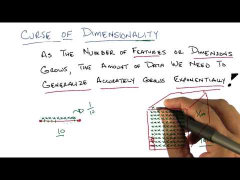
Curse of Dimensionality Two – Georgia Tech – Machine Learning
What kind of algorithm is suitable for dimensionality reduction?
The most suitable algorithm for dimensionality reduction is Principal Component Analysis (PCA). PCA is a widely used technique in data preprocessing and machine learning to transform high-dimensional datasets into lower dimensions while preserving the essential information. By reducing the number of dimensions, it helps to minimize redundant or irrelevant features, improve the efficiency of other algorithms, and reduce overfitting.
PCA works by identifying the axes with the highest variance in the data and projecting the data points onto these axes. The first principal component (PC1) captures the largest variance, while each subsequent component captures the remaining variance under the constraint that it is orthogonal to the previous components. The process continues until the desired number of dimensions is reached.
Another popular algorithm for dimensionality reduction is t-Distributed Stochastic Neighbor Embedding (t-SNE), which is particularly useful for visualizing high-dimensional data. Unlike PCA, t-SNE is a non-linear technique that is able to preserve local structures and relationships in the data. However, it can be more computationally expensive than PCA.
In conclusion, PCA is the most commonly used algorithm for dimensionality reduction, but depending on the specific use case, other techniques like t-SNE may also be suitable.
How can you select the appropriate method for dimensionality reduction?
Selecting the appropriate method for dimensionality reduction in the context of algorithms involves considering various factors, such as data type, computational complexity, and desired result. Here are some steps to follow:
1. Understand the data: Before choosing a dimensionality reduction method, it’s essential to understand the data you’re working with, including its structure and distribution.
2. Determine the goal: Identify the primary purpose of reducing dimensions, such as improving model performance, visualizing high-dimensional data, or reducing computational complexity.
3. Linear vs. non-linear methods: Consider whether your data is linearly separable or not. Linear dimensionality reduction methods like Principal Component Analysis (PCA) and Linear Discriminant Analysis (LDA) work well on linearly separable data. In contrast, non-linear methods such as t-Distributed Stochastic Neighbor Embedding (t-SNE) and Uniform Manifold Approximation and Projection (UMAP) are more suitable for non-linear data.
4. Preservation of relationships: Some dimensionality reduction techniques focus on preserving certain relationships in the data. For example, PCA preserves the maximum variance within the data, while LDA preserves class separability. Choose the method that aligns with your goals.
5. Computational complexity: Dimensionality reduction techniques have different computational complexities. Methods such as PCA and LDA are computationally efficient, whereas non-linear methods like t-SNE and UMAP can be more computationally intensive. Consider the time and resources needed to perform the chosen technique.
6. Evaluate different methods: After considering the factors above, try multiple dimensionality reduction techniques on your data and compare their results. Select the method that best achieves your objectives and meets your performance requirements.
By following these steps and taking into consideration your dataset’s specific characteristics, you can select the most appropriate method for dimensionality reduction in the context of algorithms.
Which algorithm surpasses PCA in performance?
In the context of dimensionality reduction algorithms, t-Distributed Stochastic Neighbor Embedding (t-SNE) is known to surpass Principal Component Analysis (PCA) in performance. While PCA is a linear technique, t-SNE is non-linear and can model more complex data structures. However, t-SNE comes with higher computational costs compared to PCA.
Which deep learning algorithm can be utilized for reducing dimensionality among the following options?
In the context of algorithms, among the given options, the deep learning algorithm that can be utilized for reducing dimensionality is Autoencoders. Autoencoders are a type of unsupervised neural network used to learn efficient representations of data, typically for the purpose of dimensionality reduction or feature learning. They work by compressing the input data into a lower-dimensional representation and then reconstructing the output data from this representation.
What are the top three algorithms for dimensionality reduction, and how do they differ in their approach and effectiveness?
The top three algorithms for dimensionality reduction are Principal Component Analysis (PCA), t-Distributed Stochastic Neighbor Embedding (t-SNE), and Linear Discriminant Analysis (LDA). These methods differ in their approach and effectiveness when dealing with high-dimensional data.
1. Principal Component Analysis (PCA): PCA is a linear dimensionality reduction algorithm that aims to identify the principal components or directions of maximal variance. It essentially transforms the data into a new coordinate system where the first axis corresponds to the direction of maximum variance, the second axis to the second largest variance, and so on. This method is useful in cases where linear relationships between features exist. However, PCA might not perform as well when dealing with non-linear relationships, as it only considers linear projections of the data.
2. t-Distributed Stochastic Neighbor Embedding (t-SNE): t-SNE is a non-linear dimensionality reduction technique that aims to preserve local distances between data points while reducing the dimensions. It achieves this by minimizing the divergence between two probability distributions: one representing pairwise similarities in the high-dimensional space, and the other representing pairwise similarities in the reduced-dimensional space. t-SNE is particularly effective at visualizing high-dimensional data in 2D or 3D spaces and maintains the structure of the data. However, it may be computationally expensive for large datasets.
3. Linear Discriminant Analysis (LDA): LDA is a supervised dimensionality reduction technique that uses class label information to project the data onto the most discriminative axes. It seeks to maximize class separability, which results in a better classification accuracy. LDA assumes that the data is drawn from Gaussian distributions with identical covariances for each class, and works best when these assumptions hold. However, it might not perform well when dealing with non-linear relationships, like PCA.
In summary, PCA and LDA are linear techniques that work best when underlying assumptions hold, while t-SNE is a more flexible non-linear technique suitable for visualizing complex data structures. The effectiveness of each algorithm depends on the specific problem and the structure of the data being analyzed.
How do various dimensionality reduction techniques like PCA, t-SNE, and UMAP compare in terms of computational cost and applicability in real-world scenarios?
In the context of algorithms, various dimensionality reduction techniques such as PCA (Principal Component Analysis), t-SNE (t-Distributed Stochastic Neighbor Embedding), and UMAP (Uniform Manifold Approximation and Projection) have been developed to reduce high-dimensional data to a lower-dimensional space while preserving important features and relationships. Each of these techniques has its own advantages and limitations in terms of computational cost and applicability in real-world scenarios.
PCA is a linear technique that identifies the directions of maximum variance in the dataset and projects the data onto these new axes, called principal components. This technique is computationally efficient and widely used for visualization and preprocessing purposes. However, PCA’s linear nature makes it less suitable for capturing complex, non-linear relationships in the data.
t-SNE is a non-linear technique that maps high-dimensional data points to low-dimensional counterparts in such a way that similar instances remain close together, while dissimilar ones are further apart. Although it produces visually appealing and interpretable results, t-SNE is computationally more expensive compared to PCA due to its pairwise probability calculations and can be sensitive to hyperparameters.
UMAP is another non-linear technique that aims to preserve both local and global structures in the data. It constructs a topological representation of the manifold structure and then optimizes a lower-dimensional embedding. UMAP is relatively more computationally efficient than t-SNE and is less sensitive to hyperparameters. Moreover, it can be applied to both small and large datasets, making it versatile in real-world scenarios.
In summary, PCA is preferred for its computational efficiency and simplicity, especially in cases where linear relationships suffice. t-SNE excels in producing clear visualizations but can be computationally expensive and sensitive to hyperparameters. UMAP offers a good balance between computational efficiency and preserving complex structures, making it suitable for various real-world applications. The choice of algorithm depends on the specific problem requirements, dataset size, and desired trade-offs between computation time and quality of results.
What factors should one consider when choosing the appropriate algorithm for dimensionality reduction in specific types of datasets and problem domains?
When choosing the appropriate algorithm for dimensionality reduction in specific types of datasets and problem domains, it is crucial to consider several factors:
1. Dataset Size and Structure: Some algorithms perform better on large datasets, while others are suitable for small datasets. Be aware of the dataset’s inherent structure and select algorithms that can efficiently handle that structure.
2. Computational Complexity: Dimensionality reduction methods vary in their computational complexity, which may affect the processing time and resources required. Choose an algorithm that meets the available computational resources and the desired processing time.
3. Preservation of Data Characteristics: Different algorithms emphasize preserving different aspects of data, such as global or local structures. Select a method that best captures the relevant characteristics for the given problem domain.
4. Noise Handling: The ability to separate noise from meaningful information is essential in many applications. Consider the algorithm’s robustness to noise and its ability to filter out irrelevant features.
5. Scalability: As data size increases, the scalability of the chosen algorithm becomes vital. Seek dimensionality reduction methods that can efficiently handle increasing dataset sizes without significant performance degradation.
6. Interpretability: Opt for algorithms that produce interpretable and easily understandable results, particularly when the outcome is essential for decision-making or understanding underlying patterns.
7. Application-specific Requirements: Problem-specific constraints, goals, and available prior knowledge should also guide the choice of a suitable algorithm. Some algorithms may be more adept at addressing specific challenges in certain applications or industries.
In conclusion, understanding the dataset’s characteristics and the problem context is essential when selecting the appropriate dimensionality reduction algorithm. Carefully considering factors such as dataset size, computational complexity, preservation of relevant data features, noise handling, scalability, interpretability, and application-specific requirements will help to narrow down and choose the most effective method.

